Chasing Chaos: My Journey Through Dynamic Systems and Predator-Prey Models

Figure 0: Image generated by DALL-E when I input the article you’re about to read.

Introduction

Figure 1: In a world that spawns grass slowly because of an eternal sun, this simulation visualises a rabbit population that feasts on the earth’s lettuce while foxes feast on the aforementioned rabbits. **Wait.. where are the foxes?**

Imagine a GIF where foxes and rabbits dart across the screen in a simulated ecosystem, each move calculated by complex algorithms. This visual is more than just digital art; it’s a glimpse into the sophisticated world of computational ecology explored in one of my Master’s modules at the University of Sheffield. This project bridges the gap between theoretical biology and applied computational techniques by extending the classical predator-prey models of Lotka and Volterra and incorporating the chaotic dynamics of the Duffing Oscillator.

How did I make it a realistic simulation?

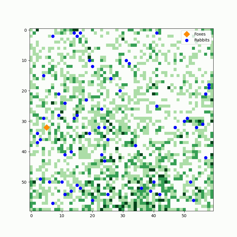
Realism was added in two elements: a good model of animal populations and interactions and good agent-based modelling (ABM). Through an ABM approach, each agent (animal) followed specific behavioural rules and had specific properties (to be shown later), which provided insights into the complexity of ecological dynamics.

Understanding the Lotka-Volterra Equations

The foundational work by Alfred J. Lotka and Vito Volterra has been pivotal in ecological modelling. Their predator-prey equations, which describe the interactions between species, served as the starting point for my analysis. This project provided an opportunity to apply these classic models and extend them using modern computational techniques, and, to of course, make cool visualisations.

The Lotka-Volterra equations are a pair of first-order, nonlinear, differential equations that describe the dynamics of biological systems in which two species interact, one as a predator and the other as prey. Here’s a simplified breakdown of the equations:

$\text{Prey Population Growth:} \quad \frac{dx}{dt} = \alpha x - \beta xy$

Where:

(x) is the number of prey.
(\alpha) is the natural growth rate of the prey in the absence of predation.
(\beta) represents the rate of predation—how often the predators successfully capture the prey.

$\text{Predator Population Decline and Growth:} \quad \frac{dy}{dt} = \delta xy - \gamma y$

Where:

(y) is the number of predators.
(\delta) represents the growth rate of the predator population due to successful hunts—how feeding on the prey increases the predator population.
(\gamma) is the natural decline rate of predators in the absence of sufficient prey.

The Role of RK4 in Simulating These Dynamics

To simulate these complex interactions, I employed the RK4 method—a numerical technique used to solve ordinary differential equations. RK4 is particularly well-suited for dealing with the complexities of biological models because it provides a good balance between computational efficiency and accuracy. It does its business by calculating the populations of predators and prey at successive steps, offering a detailed picture of how these populations change over time due to various biological factors.

So what did I do?

Using Python, I implemented these equations to create simulations illustrating the potential outcomes of predator-prey interactions under different ecological conditions. These simulations help us visualize scenarios such as what happens if the prey population grows too large or if predators overhunt their prey. It’s a dynamic representation that informs ecological understanding and highlights the importance of balance in natural ecosystems.

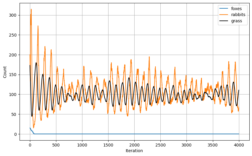
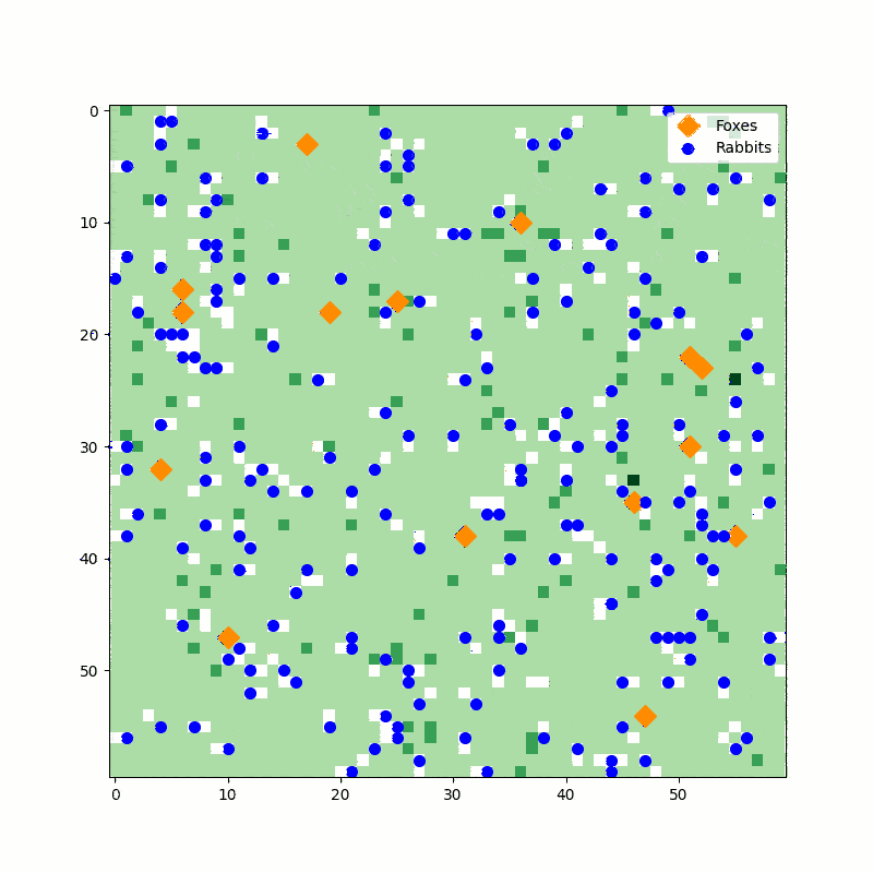
In my environment, each animal was assigned a speed attribute, a vision attribute, and an attribute that dictated the minimum energy needed to reproduce. Based on this, in my research, I made three different scenarios where I tweaked the fox (predator) vision attribute to investigate the difference in the environment dynamics of each fox attribute:

Scenario 1: The foxes can only sense animals that are one square in any direction.

The population graphs are shown in the following figure, and the simulation is visualised in the preceding figure.

Result: Unsustainable Ecosystem.
Cause: Foxes died too early.

Scenario 2: The foxes can only sense animals that are a maximum of four squares in any direction.

The population graphs are shown in the following figure, and the simulation is visualised in the preceding figure.

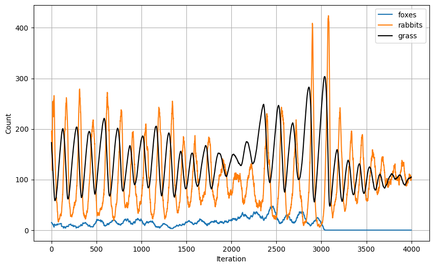
Result: For a while, the ecosystem was stable but eventually unsustainable.
Cause: Foxes died out later due to over-predation at around iteration 2400, followed by a volatile period of population increase and decrease, which was terrible for ecosystem health and eventually led to the foxes not finding enough rabbits to eat, resulting in their extinction.

Scenario 2’s GIF file is available at the bottom.

Scenario 3: The foxes can only sense animals that are seven squares in any direction.

The population graphs are shown in the following figure, and the simulation is visualised in the preceding figure.

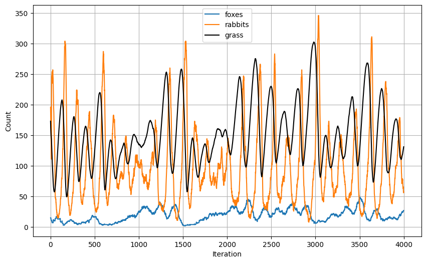
Result: Sustainable Ecosystem.
Cause: While volatile rabbit and grass population phases still occurred here, the foxes recovered quickly due to their better sense of sight. This allows for a balanced ecosystem to exist due to the foxes now having a key predator-like attribute, providing them with the natural “unfair” advantage over prey.

Scenario 3’s GIF file is available at the bottom.

Conclusion

The Lotka-Volterra models, enhanced by the precision of the RK4 simulation method, provide a powerful tool for understanding and predicting the behaviors of interacting species. This project not only deepened my appreciation for the complexity of natural systems but also demonstrated how mathematical modeling can be a gateway to understanding the rhythms of life that govern our planet.

Ready to dive deeper? You can explore the interactive simulations and detailed analysis in the complete Jupyter Notebook available at the bottom of the screen. Whether you’re a budding ecologist, a seasoned data scientist, or simply curious about nature’s intricacies, these simulations offer a window into the fascinating world of ecological dynamics.

Yousef Qasim